Problem Set 6. DID + synthetic control
Relevant material will be covered by Nov 9. Problem set is due Nov 16.
To complete the problem set, feel free to Download the .Rmd. Omit your name so we can have anonymous peer feedback. Submit the PDF on Canvas.
The learning goals of completing this problem set are to engage with conceptual assumptions for difference in difference and synthetic control.
1. (25 points) Difference in Difference
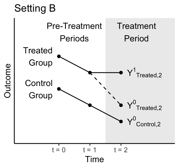
In the figures below, the treated group becomes treated between time 1 and time 2. The control group never becomes treated. Figures are hypothetical scenarios that depict true potential outcomes even if those outcomes would not be observed in an actual study.

1.2 (5 points)
In actual data analysis, can we ever know for certain whether we are in Setting A or Setting B? If the answer is no, then tell us which outcome cannot be observed.
1.3 (5 points)
A researcher comes to you with the data below, which depict only observed outcomes. That researcher wants to run a difference in difference analysis. Here, we have not depicted the counterfactual outcome because the researcher would not know it.
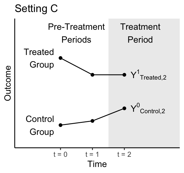
Why is the parallel trends assumption doubtful in this setting?
1.4 (5 points)
A researcher is interested in the causal effect of a minimum wage increase on employment. They plan to study only the U.S., and they are interested in a time when the minimum wage rose simultaneously at every place in the U.S. Why won’t a difference in difference design work for the researcher’s question?
2. (25 points) Synthetic Control
In discussion, we considered the paper by Abadie and Gardeazabal (2003) which estimates the effect of terrorist conflict in the Basque Country on GDP per capita. Using synthetic control, they construct a synthetic version of Basque Country. We show the selected weights and plot the gap between the observed and synthetic Basque Country below.
##    w.weights                   unit.names unit.numbers
## 2      0.000                    Andalucia            2
## 3      0.000                       Aragon            3
## 4      0.000       Principado De Asturias            4
## 5      0.000             Baleares (Islas)            5
## 6      0.000                     Canarias            6
## 7      0.000                    Cantabria            7
## 8      0.000              Castilla Y Leon            8
## 9      0.000           Castilla-La Mancha            9
## 10     0.851                     Cataluna           10
## 11     0.000         Comunidad Valenciana           11
## 12     0.000                  Extremadura           12
## 13     0.000                      Galicia           13
## 14     0.149        Madrid (Comunidad De)           14
## 15     0.000           Murcia (Region de)           15
## 16     0.000 Navarra (Comunidad Foral De)           16
## 18     0.000                   Rioja (La)           18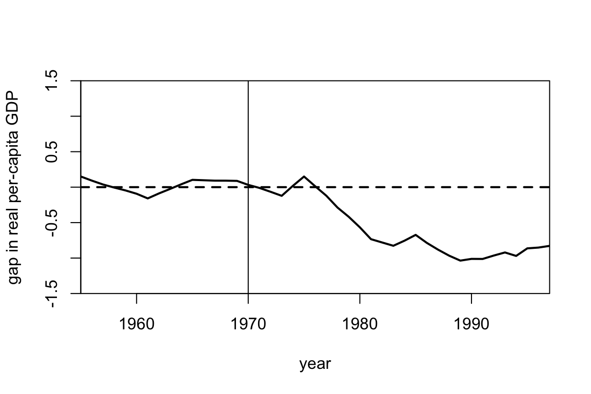
2.1 (10 points) Motivation
Instead of selecting the weights using synthetic control, we could have instead estimated the potential outcome for Basque Country using a regression approach. Specifically, we consider the data prior 1970 and simply regress the GDP per capita in the Basque region onto the GDP per capita in other regions to find coefficients \(\hat \beta\) so that \[\widehat{Y^{0}}_{t, Basque} = \sum_j \hat \beta_{j} Y^{0}_{t, j}.\] We then use the estimated \(\hat \beta\) to predict \(\widehat{Y^{0}}_{t, Basque}\) after treatment occurs. The weights and gap plot are shown below. We haven’t included all the regions in the code below, but you don’t need to worry about that.
Looking at the estimated weights sand the gap plots, why might you prefer the synthetic control estimate over the regression based estimate? Why might you prefer the regression estimate over the synthetic control estimate?
##   weights                         name id
## 1  -0.632                       Aragon  3
## 2   1.256       Principado De Asturias  4
## 3  -0.586             Baleares (Islas)  5
## 4   0.438                    Cantabria  7
## 5   0.594                     Cataluna 10
## 6  -0.788         Comunidad Valenciana 11
## 7   0.155        Madrid (Comunidad De) 14
## 8  -0.245 Navarra (Comunidad Foral De) 16
## 9   1.136                   Rioja (La) 18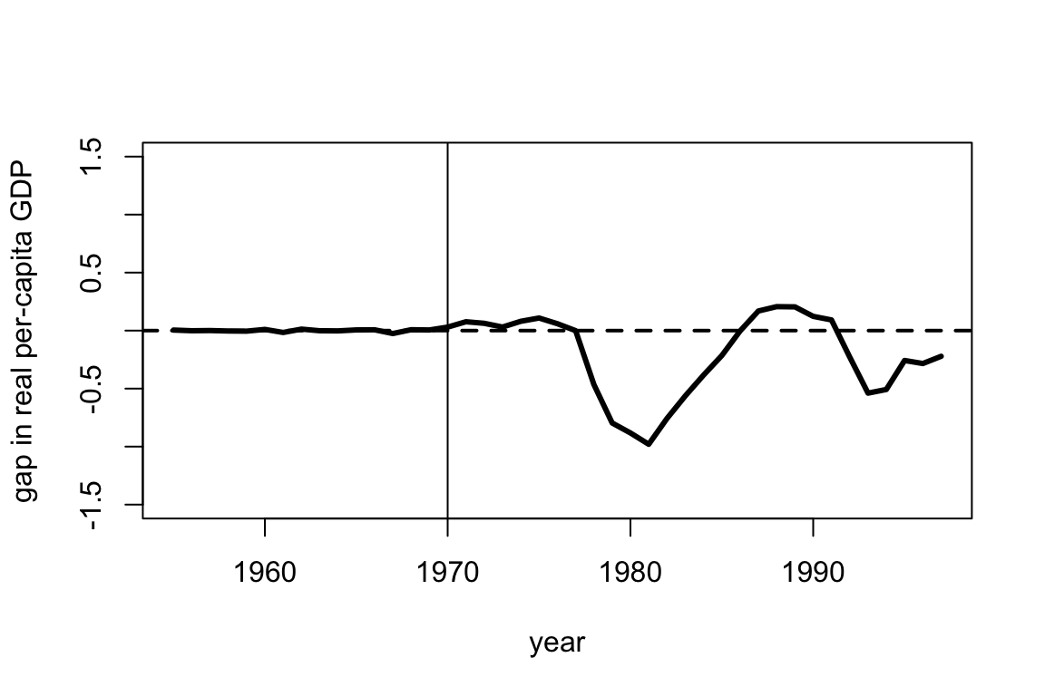
2.2 (5 points) Assessing fit
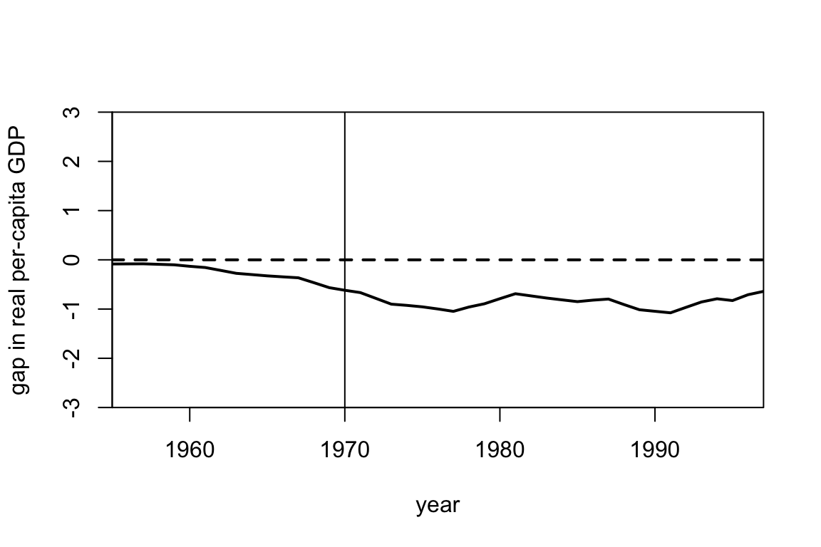
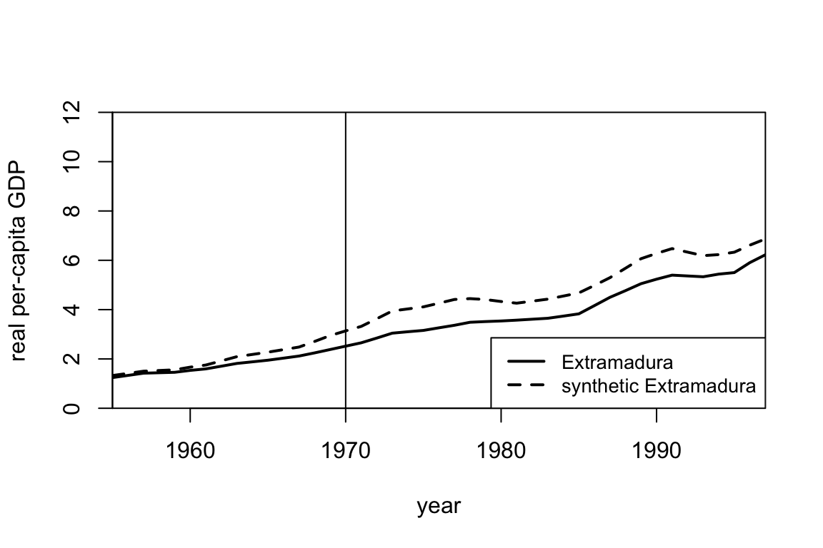
Using the same dataset, suppose we wanted to estimate the causal effect for some policy implemented in Extramadura (another region in Spain) in 1970. Running synthetic control gives an estimate of almost -1000 dollars in 1990. Looking at the plots below, why might you be skeptical of the resulting estimate?
2.3 (5 points) Hypothesis testing
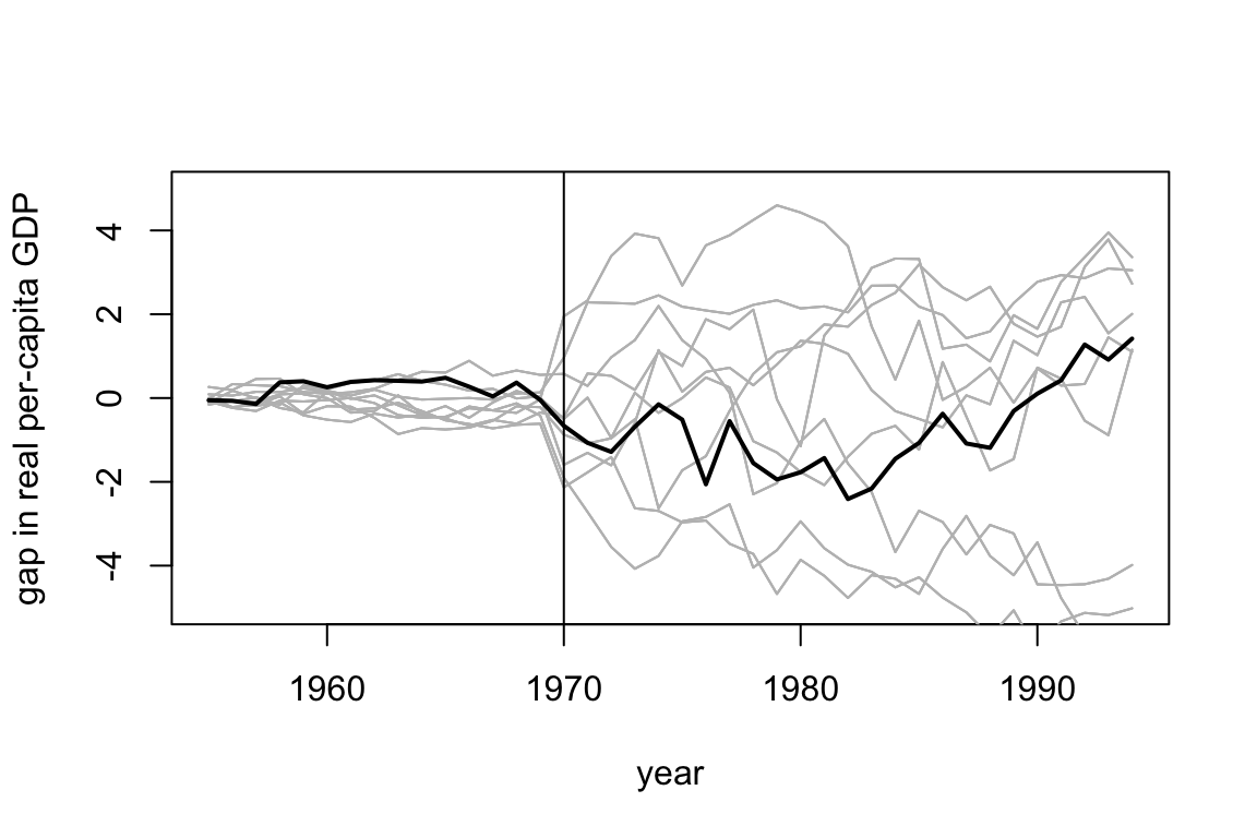
Suppose we used synthetic control for each of the other regions in Spain as a placebo test. Below, we show a hypothetical plot for the gap between the observed and synthetic values for each region. The difference between observed and synthetic Basque country is shown in the dark black line and the others are shown in gray. Note this is made up data. However, if this were the real plot you saw, would you be confident that there was a non-zero causal effect for Basque Country? Explain why or why not.
2.4 (5 points) Interference
It’s reasonable to believe that the effect of the terrorist conflict might spillover onto neighboring regions as well. Suppose the economy of Basque country is very intertwined with the economy of neighboring regions, and when we estimate a synthetic Basque country, the weights for neighboring regions are large. If the terrorist conflict also has a negative effect on the neighboring regions but we don’t account for it in our analysis, how would this effect the estimated causal effect?