Problem Set 5. IV + RD
Relevant material will be covered by Oct 26. Problem set is due Nov 2.
To complete the problem set, feel free to Download the .Rmd. Omit your name so we can have anonymous peer feedback. Submit the PDF on Canvas.
The learning goals of completing this problem set are to engage with conceptual assumptions for instrumental variables and regression discontinuity.
1. (20 points) Instrumental variables in experiments
Suppose you are an elementary school principal. You randomize some students to a new program to receive extra tutoring at an off-site location in the evenings. You randomize other students to a no-tutoring condition.
In many cases, students’ treatment assignments \(Z\) determines their actual treatments \(A\) (when \(Z = 1\) then \(A = 1\), and when \(Z = 0\) then \(A = 0\)). But there are some difficulties:
- The parents of some students work evenings and can’t drive their children to the tutoring (\(U\)). No matter the value of \(Z\), these children do not receive tutoring (\(A = 0\)).
- The parents of some students make a huge fuss (\(U\)) so that regardless of the value of \(Z\), these parents ensure that their children receive tutoring (\(A = 1\)).
Answer the following in a sentence each.
- (3 points) What is the intent to treat effect?
- (3 points) Who are the always-takers?
- (3 points) Who are the never-takers?
- (3 points) Who are the compliers?
- (3 points) Although they are not discussed above, describe how someone could be a defier.
- (5 points) What assumption was made credible by randomization of \(Z\)?
2. (10 points) IV in observational studies
Much of the water supply for the state of California comes from snowmelt in the Sierra Nevada Mountains. Two economists are very excited to notice that some years have much larger snowpacks than others—this could be an instrument!
Economist 1
Economist 2
The first economist argues that random differences in the Sierra snowpack create random fluctuations in agricultural productivity, thereby providing an instrumental variable for the effect of agricultural productivity on the state’s GDP.
The second economist argues that random difference in the Sierra snowpack create random fluctuations in the quality of skiing at Mammoth Mountain and other Sierra resorts, thereby providing an instrumental variable for the effect of ski resort productivity on the state’s GDP.
Both economists argue that their instruments are valid because the snowpack is randomly assigned. Can both economists be right that their instrument is valid? Why or why not?
3. (20 points) Regression discontinuity
3.1 (5 points) A local estimand
A colleague tells you they’ve read that regression discontinuity designs have proven that winning one election (greater than 50% of the vote) causes a political party to have better chances in the next election. In your district, the winner won with 70% of the vote. Why isn’t the regression discontinuity evidence very informative for districts like yours?
3.2 (5 points) Examples of Discontinuity
Describe an example you have encountered where a regression discontinuity analysis might be used to estimate a causal effect. Draw a causal diagram for the example.
3.3 (10 points) Effect of incumbency
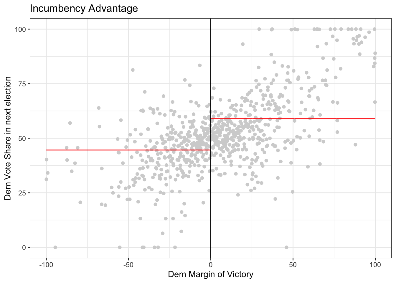
In the discussion section, we considered two causal effects. First, we estimated the causal effect of incumbency when a senator is up for re-election. Next, we considered the causal effect of the senator who is not up for election being a democrat on the democratic vote share of the senator who is up for election.
Using the package, give an estimate for the second causal effect. Also, explain the results by clearly stating the quantity we are estimating in plain language and also explaining whether you conclude that the causal effect is non-zero or not.
### Code from Discussion section to get you started

library(ggplot2)
library(rddensity)
library(rdrobust)
library(rdlocrand)

data <- read.csv("https://raw.githubusercontent.com/rdpackages-replication/CIT_2020_CUP/master/CIT_2020_CUP_senate.csv")

dem_vote_t1 <- data$demvoteshfor1
dem_margin_t0 <- data$demmv

# plotting the data
# Shows average to the left and to the right of the cut-off
rdplot(y = dem_vote_t1,
       x =  dem_margin_t0, nbins = c(1000, 1000),
       p = 0, col.lines = "red",
       col.dots = "lightgray",
       title = "Incumbency Advantage",
       y.lim = c(0,100),
       x.label = "Dem Margin of Victory",
       y.label = "Dem Vote Share in next election")