Discussion 07. Causal Effects with Matching
NOTE: This is from Fall 2023. We have not updated to reflect the current term yet.
Slides Download today’s .Rmd document here.
Some packages you may need to install first:
- optmatch:
install.packages("optmatch") - sandwich:
install.packages("sandwich") - MatchIt:
install.packages("MatchIt") - marginaleffects:
install.packages("marginaleffects")
13.7 R Markdown
Learn to do matching with the “MatchIt” package
First, we’ll use the data set from last week to compare greedy vs optimal matching. We’ll use the NLSY data since it is larger.
d <- readRDS("assets/discussions/d.RDS")

# matchit function implements matching
# Formula: Treatment ~ variables to match on
# method: nearest is a greedy 1:1 matching without replacement
# distance: euclidean (other possible options are scaled_euclidean, mahalanobis, robust_mahalanobis)
# read more on distances here: https://rdrr.io/cran/MatchIt/man/distance.html#mat
m.out0 <- matchit(a == "college" ~ log_parent_income + log_parent_wealth
                              + test_percentile,
                              method = "nearest", distance = "euclidean",
                              data = d)
First compare optimal vs greedy. Optimal matching is usually better than greedy matching, as long as your data isn’t too big
## Optimal vs greedy with NYLSR data
# With n = 1000; .01 sec vs .8 sec
# With n = 2000; .05 sec vs 8 sec
# With n = 4000; .1 vs 25

ind <- sample(nrow(d), size = 1000)

# Greedy is using nearest
system.time(m.out0 <- matchit(a == "college" ~ log_parent_income + log_parent_wealth
                              + test_percentile,
                              method = "nearest", distance = "euclidean",
                              data = d[ind, ]))
## user system elapsed
## 0.016 0.000 0.016
# method: optimal is optimal matching
system.time(m.out0 <- matchit(a == "college" ~ log_parent_income + log_parent_wealth
                              + test_percentile,
                              method = "optimal", distance = "euclidean",
                              data = d[ind, ]))
## user system elapsed
## 1.290 0.077 1.524On the full data, using optimal is possible, but can take a bit of time. On larger data sets, it might not be possible
# With full data set greedy matching takes ~ 0.5-1.5 seconds
system.time(m.out0 <- matchit(a == "college" ~ log_parent_income + log_parent_wealth
                              + test_percentile,
                              method = "nearest", distance = "euclidean",
                              data = d))
## user system elapsed
## 0.605 0.077 0.684
# Meanwhile, optimal matching takes 60-130 seconds
system.time(m.out0 <- matchit(a == "college" ~ log_parent_income + log_parent_wealth
                              + test_percentile,
                              method = "optimal", distance = "euclidean",
                              data = d))
## user system elapsed
## 117.511 5.250 124.21513.8 Matching with job training data from “Evaluating the econometric evaluations of training programs with experimental data” (LaLonde 1986)
For the remainder of the lab, we’ll use a portion of the data from a job training program. In particular, the treatment is whether or not someone participated in a job training program. The outcome of interest is their salary in 1978 (re78).
# Load the data
data("lalonde")

# See what's in the data
?lalonde # this opens up the "Help" tab with the documentation!
head(lalonde)
## treat age educ race married nodegree re74 re75
## NSW1 1 37 11 black 1 1 0 0
## NSW2 1 22 9 hispan 0 1 0 0
## NSW3 1 30 12 black 0 0 0 0
## NSW4 1 27 11 black 0 1 0 0
## NSW5 1 33 8 black 0 1 0 0
## NSW6 1 22 9 black 0 1 0 0
## re78
## NSW1 9930.0460
## NSW2 3595.8940
## NSW3 24909.4500
## NSW4 7506.1460
## NSW5 289.7899
## NSW6 4056.4940We expect income in 1974 is highly correlated with income in 1975. It also has a much higher variability than age.
## Suppose there are 3 individuals
dat <- matrix(c(50, 5000, 5500,
                20, 5100, 5900,
                40, 5200, 6200), ncol = 3, byrow = T)
colnames(dat) <- c("age", "re74", "re75")

# Is individual 2 or 3 more similar to individual 1?
# To answer this, we should compute the distances between individuals 1 and 2, and 1 and 3.

# One way is to compute the Mahalanobis distance by first computing the covariance matrix of the confounding variables
# In this case, the confounders are age, re74, and re75
dataCov <- lalonde %>%
  select(age, re74, re75) %>%
  cov

# Then we compute the Mahalanobis distance with the function mahalanobis_dist
mahalanobis_dist( ~ age + re74 + re75, data = dat, var = dataCov)
## 1 2 3
## 1 0.000000 3.225953 1.098595
## 2 3.225953 0.000000 2.152528
## 3 1.098595 2.152528 0.000000
# We can also compute the Euclidean distance
dist(dat, method = "euclidean")
## 1 2
## 2 413.4005
## 3 728.0797 316.8596Now let’s try to run the matching procedure using the function.
# For now, let's start with Euclidean distance, even if may not be great

# method: nearest (i.e. greedy 1:1)
# distance: euclidean
# data: lalonde (the data set we're working with)
# replace: True (T) or False (F) - whether to sample with or without replacement.
    # Note, if allowing for replacement, greedy and optimal are the same
    # So for the function, you only need to specify if using method = "nearest"
# ratio: how many control matches for each treated unit
# caliper: by default, the caliper width in standard units (i.e., Z-scores)
m.out0 <- matchit(treat ~ re74 + re75 + age + race,
                  method = "nearest", distance = "euclidean",
                  data = lalonde, replace = F,
                  ratio = 1, caliper = c(re74  = .2, re75 = .2))
13.9 Assessing the matching
We can check how well the balancing has been done
?summary.matchit # Look in the Help tab (on the bottom right) for documentation on summary.matchit


# interactions: check interaction terms too? (T or F)
# un: show statistics for unmatched data as well (T or F)
summary(m.out0, interactions = F, un = F)
##
## Call:
## matchit(formula = treat ~ re74 + re75 + age + race, data = lalonde,
## method = "nearest", distance = "euclidean", replace = F,
## caliper = c(re74 = 0.2, re75 = 0.2), ratio = 1)
##
## Summary of Balance for Matched Data:
## Means Treated Means Control Std. Mean Diff.
## re74 1643.2931 1666.9106 -0.0048
## re75 1021.5989 1086.1734 -0.0201
## age 25.6971 26.1543 -0.0639
## raceblack 0.8400 0.2800 1.5403
## racehispan 0.0571 0.1714 -0.4833
## racewhite 0.1029 0.5486 -1.5040
## Var. Ratio eCDF Mean eCDF Max Std. Pair Dist.
## re74 1.0122 0.0108 0.1543 0.0293
## re75 1.0026 0.0166 0.1543 0.0422
## age 0.4213 0.0894 0.2000 0.9967
## raceblack . 0.5600 0.5600 1.7289
## racehispan . 0.1143 0.1143 0.7249
## racewhite . 0.4457 0.4457 1.6968
##
## Sample Sizes:
## Control Treated
## All 429 185
## Matched 175 175
## Unmatched 254 10
## Discarded 0 0
# Std. Mean Diff (SMD): difference of means, standardized by sd of treatment group
# Var. Ratio: ratio of variances in treatment and control group. Compares spread of data
# Rubin (2001) presents rule of thumb that SMD should be less than .25 and variance ratio should be between .5 and 2
# Max eCDF: Kolmogorov-Smirnov statistic. Max difference across entire CDF
We can also visually asses the matches
## Produces QQ plots of all variables in which.xs
plot(m.out0, type = "qq", which.xs = ~age + re74, interactive = F)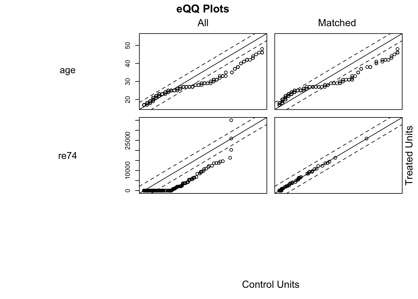
## Plots the density of all variables in which.xs
plot(m.out0, type = "density", which.xs = ~age + re74 + race, interactive = F)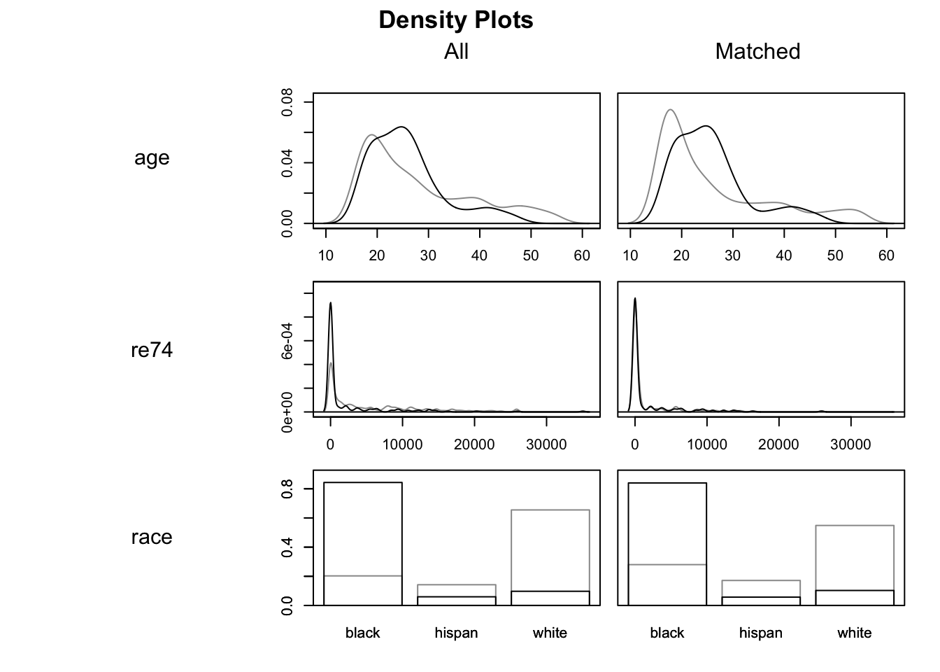
## Plots the empirical CDF of all variables in which.xs
plot(m.out0, type = "ecdf", which.xs = ~age + re74, interactive = F)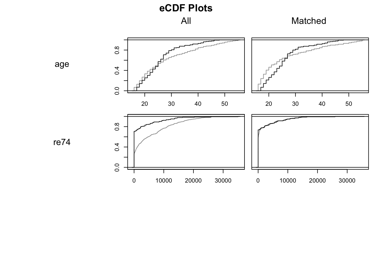 ## Estimating the effect
Given the matching (and assuming it is good enough), we can estimate the ATT.
## Estimating the effect
Given the matching (and assuming it is good enough), we can estimate the ATT.
# Produces data frame same as input, but has two additional columns
# weights: the weight of the row in the paired data set. Can be greater than 1
#         if the data set was matched more than once
# subclass: the index of the "pair"
#
m.out0.data <- match.data(m.out0, drop.unmatched = T)
head(m.out0.data)
## treat age educ race married nodegree re74 re75
## NSW1 1 37 11 black 1 1 0 0
## NSW2 1 22 9 hispan 0 1 0 0
## NSW3 1 30 12 black 0 0 0 0
## NSW4 1 27 11 black 0 1 0 0
## NSW5 1 33 8 black 0 1 0 0
## NSW6 1 22 9 black 0 1 0 0
## re78 weights subclass
## NSW1 9930.0460 1 1
## NSW2 3595.8940 1 88
## NSW3 24909.4500 1 99
## NSW4 7506.1460 1 110
## NSW5 289.7899 1 121
## NSW6 4056.4940 1 132
names(m.out0.data)## [1] "treat" "age" "educ" "race" "married"
## [6] "nodegree" "re74" "re75" "re78" "weights"
## [11] "subclass"
# Also produces matched data set, though will duplicate rows if matching with replacement
# and a control is matched more than once
m.out0.data <- get_matches(m.out0)
As a first step, we could simply compare the means of the outcomes for both groups. Notice this is the first time we’ve looked at the outcomes!
# Take the mean of both groups
# this will only work if all weights are 1
aggregate(re78~ treat, FUN = mean, data = m.out0.data)
## treat re78
## 1 0 5422.184
## 2 1 6193.594
# Fitting a linear model on the treatments will work
# even if all weights are not 1. We just need to feed them in
fit1 <- lm(re78~ treat, data = m.out0.data, weights = weights)

# vcov: tells R to use robust standard errors
avg_comparisons(fit1, variables = "treat",
                vcov = "HC3",
                newdata = subset(m.out0.data, treat == 1),
                wts = "weights")
## Warning: The `treat` variable is treated as a categorical
## (factor) variable, but the original data is of class
## integer. It is safer and faster to convert such
## variables to factor before fitting the model and
## calling `slopes` functions.
##
## This warning appears once per session.##
## Term Contrast Estimate Std. Error z Pr(>|z|) S 2.5 %
## treat 1 - 0 771 753 1.02 0.306 1.7 -705
## 97.5 %
## 2248
##
## Columns: term, contrast, estimate, std.error, statistic, p.value, s.value, conf.low, conf.high
## Type: response13.10 Fit your own model
Now try for yourself. Note, you will need to do something very similar for the homework with this dataset.
- Think about what an appropriate DAG might be and choose the variables you want to match on
- Ask yourself: Do I know how to choose variables I should match on?
- Choose a matching procedure
- Ask yourself: Do I know how to explain this matching procedure and its bias-variance trade off?
- Evaluate the balance in the match. If it doesn’t look good, try another matching procedure
- Ask yourself: Do I know what a balanced matching looks like?
- Estimate the causal effect
- Ask yourself: Do I know what I just estimated?