Problem Set 4. Statistical Modeling
Relevant material will be covered by Oct 16. Problem set is due Oct 27.
To complete the problem set:
- Copy and Paste this into a .Rmd file and complete the homework.
- Omit your name so we can have anonymous peer feedback. Compile to a PDF and submit the PDF on Canvas.
This problem set uses data from the following paper:
Dehejia, R. H. and Wahba, S. 1999. Causal Effects in Nonexperimental Studies: Reevaluating the Evaluation of Training Programs. Journal of the American Statistical Association 94(448):1053–1062.
The paper compares methods for observational causal inference to recover an average causal effect that was already known from a randomized experiment. You do not need to read the paper; we will just use the study’s data as an illustration.
The following lines will load these data into R.
## ── Attaching core tidyverse packages ──── tidyverse 2.0.0 ──
## ✔ dplyr     1.1.4     ✔ readr     2.1.5
## ✔ forcats   1.0.0     ✔ stringr   1.5.2
## ✔ ggplot2   4.0.0     ✔ tibble    3.3.0
## ✔ lubridate 1.9.4     ✔ tidyr     1.3.1
## ✔ purrr     1.0.4
## ── Conflicts ────────────────────── tidyverse_conflicts() ──
## ✖ dplyr::filter() masks stats::filter()
## ✖ dplyr::lag()    masks stats::lag()
## ℹ Use the conflicted package (<http://conflicted.r-lib.org/>) to force all conflicts to become errors## randomForest 4.7-1.2
## Type rfNews() to see new features/changes/bug fixes.
##
## Attaching package: 'randomForest'
##
## The following object is masked from 'package:dplyr':
##
## combine
##
## The following object is masked from 'package:ggplot2':
##
## margin
data("lalonde")1. (10 points) Drawbacks of Exact Matching
In the discussion section on Wednesday, October 15th, you walked through an example of exact matching with high-dimensional confounding. You looked at some statistics and information of the re74 values in the full data versus the matched data. Answer the following questions about what you observed:
- Notice the difference between the values of re74 in the full data versus the matched data. Explain what happened and why it happened.
- In light of this example, what is the drawback of using exact matching in this type of setting?
Answer.
2. (10 points) Outcome modeling with Parametric G-formula
In the code below, we use randomForest to learn a model of future earnings re78 on treatment treat, interacted with confounders: race, ‘age’, married, nodegree, and re74. A random forest is a machine learning method that trains multiple decision trees in the final prediction model.
Knowing about decision trees and random forests is not necessary for this course or problem set. However, if you are interested in learning more about these machine learning methods, you can take a look at this cool (and free) Google course or watch this short video from IBM Technology. Documentation for the R Library
randomForestcan be found here. Random forests have a random element when fitting the model. That means each time you re-run the code, the answer may be slightly different. To fix the result to a specific value, we will use the code `set.seed(111)’
# set the random number generator to a specific state
set.seed(111)

# fit the outcome model using random forests
outcome_model <- randomForest(re78 ~ treat*(race + age +married + nodegree + re74),
                              data = lalonde)
YOUR TASK: Use the model above to estimate the average treatment effect among the treated (the ATT). To make your code easier to grade, break this task into the following three steps:
- Create two data frames from the
lalondedata:- The first should contain the treated individuals (with their factual treatment of
1) - The second should contain the same treated individuals, but with
treatset to the value0. - Hint: Both data frames should only contain individuals who were actually treated. One way to do this is with the
filterfunction.
- The first should contain the treated individuals (with their factual treatment of
- Using the
outcome_modelabove, predict the expected outcomes for the two data frames you created in step 1. - Report the average treatment effect among the treated (ATT).
# Your code goes here3. (10 points) IPW estimator
Alternatively, we could use a propensity score model to estimate the Average Treatment effect (on everyone, not just those who are treated).
propensity_scores <- glm(treat ~race + age +married + nodegree + re74, family = binomial, data = lalonde)YOUR TASK: Use the model above to estimate the average treatment effect among everyone (the ATE).
# Your code goes here4. Choosing a distance metric for matching
To better understand the importance of choosing a distance metric we will consider only a subset of the lalonde data. We will choose a match for an individual in the treatment group based on age and re74.
lalonde_sub <-
  lalonde[c("NSW185","PSID250","PSID303"),] %>%
  select(treat,age,re74) %>%
  data.frame(row.names= c("Ind1", "Ind2", "Ind3"))

lalonde_sub_0 <-
  lalonde_sub %>%
  filter(treat==0)

print(lalonde_sub)
## treat age re74
## Ind1 1 33 14660.71
## Ind2 0 32 12553.02
## Ind3 0 52 14780.714.1. (1 point) Getting intuition
By looking at the table above and the histograms of the variables below, do you think Ind2 or Ind3 would be a better match with Ind1? Why?
hist(lalonde$age)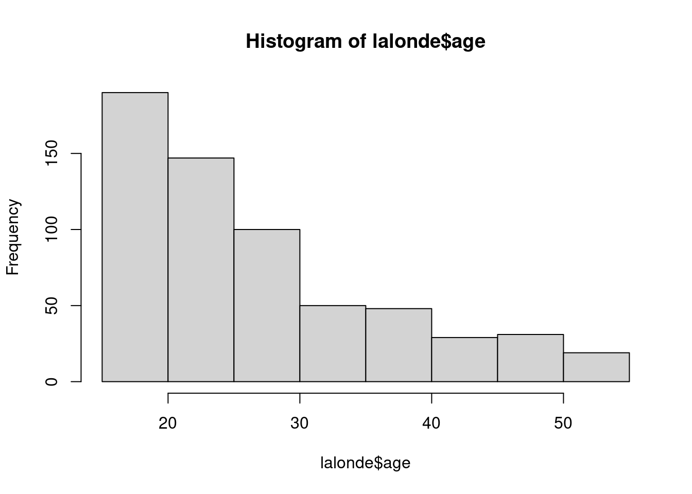
hist(lalonde$re74)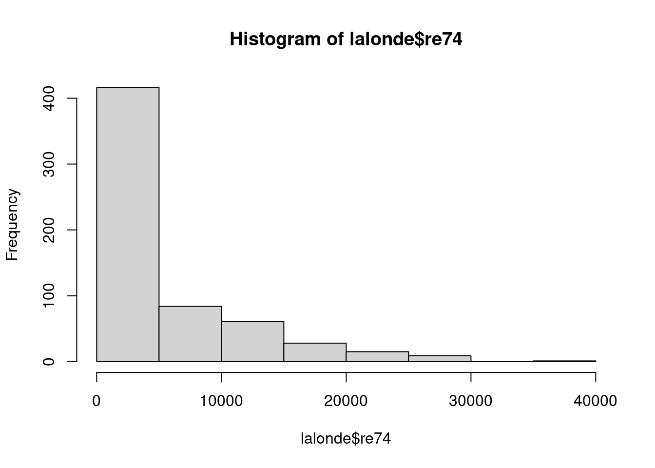
4.2. (5 points) Euclidean distance
Using the euclidean distance, which individual would be the closest match with Ind1?
Remember the euclidean distance is given by \(d(i,j) = \sqrt{\sum_p \left( L_{pi} - L_{pj}\right)^2}\). Fill in the missing variables (indicated by ...) to calculate the euclidean distance:
age_ind1 = lalonde_sub["Ind1","age"]
re74_ind1 = lalonde_sub["Ind1","re74"]


# Uncomment the code below by taking away the # at the beginning of each line
# then fill out the ...

# lalonde_sub_0 %>%
#  mutate(age_dif= ...,
#         re74_dif = ...,
#         euc_dis = sqrt(...)) %>%
#  select(euc_dis)
4.3. (5 points) Mahalanobis distance
Using the Mahalanobis distance, which individual would you match with Ind1?
Remember the Mahalanobis distance adjusts for the fact that some variables are measured on different scales than others. Thus, for each variable the distance is divided by the standard deviation of the variable. Furthermore, it adjusts for correlations within variables as well. Mathematically, it is given by \(d(i, j) =\sqrt{(\vec{L}_i -\vec{L}_j)^T\Sigma^{-1}(\vec{L}_i -\vec{L}_j)}\), where \(\Sigma\) is the covariance of \(\vec{L}\).
Fill in the missing variables (indicated by ...) to calculate the mahalanobis distance. Note that we’re using the function solve() to get the inverse of a matrix.
## the contrivance matrix for age and re74 based on the entire dateset:
Sigma = cov(lalonde[,c("age","re74")])

# standard deviation of age
sqrt(Sigma[1,1])
## [1] 9.881187
# standard deviation of income in 1974
sqrt(Sigma[2,2])
## [1] 6477.964
# Uncomment the code below by taking away the # at the beginning of each line
# then fill out the ...

#lalonde_sub_0 <-
#  lalonde_sub_0 %>%
#  mutate(age_dif= ...,
#         re74_dif = ...)
# L <- as.matrix(lalonde_sub_0[,c("age_dif","re74_dif")]) # the matrix of differences


# Uncomment the code below by taking away the # at the beginning of each line
# then fill out the ...

# m_dis_ind2 <- sqrt(L["Ind2",] %*% solve(Sigma) %*%  L["Ind2",])
# m_dis_ind3 <- ...
# m_dis <- c("Ind2" = m_dis_ind2, "Ind3" = m_dis_ind3)
# print(cbind(m_dis))5. Matching without requiring exact matches
We hope that from this class you are prepared to learn new causal estimators, apply them in R, and explain what you have done. This question is a chance to practice! In class we discussed many matching approaches. For this question, you will choose your own approach. There are many correct answers, and you will be evaluated by the clarity of your code and explanations.
Task: Using matchit, conduct matching to estimate the ATT where treat is the treatment and the sufficient adjustment set is race, married, nodegree, and re74.
- Use
matchit, settingmethod,distance, and any other arguments (likereplace,caliper,ratio) to any values of your choosing. The only requirements areformula = treat ~ race + age + married + nodegree + re74estimand = "ATT"- For
method, you may not useexact.
- Create matched dataset using
match.data() - Using linear regression with
lm(), estimate a model using the formulare78 ~ treat*(age + race + married + nodegree + re74)and your matched data, weighted by theweightsthat are produced bymatch.data(). - Report your estimate of the ATT.
5.1. (5 points) Conduct the matching
This is space to conduct the matching. We expect this part to be an R code chunk.
# Your code goes here6. (10 points) Reflection Question
Answer the following two questions in a short paragraph. For full credit, you must refer to at least two lecture or discussion slides or exercises that relate to what you choose to write about (at least one for each part). To cite slides, simply reference the slide number and date. If you are citing an exercise/.Rmd notebook from a discussion or lecture, indicate the date, title, and subsection if appropriate.
Reflect on your overall experience in the course so far by describing an interesting idea or tool you learned, why it was interesting to you, and what it tells you about causal inference.
Reflect on your overall experience with the course so far by telling us about a particular topic/question that you found challenging, why it was hard for you, how you approached the problem, and what you learned by struggling through the problem.
Answer.