Discussion 8. Matching
STSCI/INFO/ILRST 3900: Causal Inference
October 15, 2025
You can download the slides for this week’s discussion and the .Rmd.
The first exercise and problem set 4 use the lalonde dataset from the following paper:
Dehejia, R. H. and Wahba, S. 1999. Causal Effects in Nonexperimental Studies: Reevaluating the Evaluation of Training Programs. Journal of the American Statistical Association 94(448):1053–1062.
The paper compares methods for observational causal inference to recover an average causal effect that was already known from a randomized experiment. You do not need to read the paper; we will just use the study’s data as an illustration. We’ll load the data into R with the first code block.
To learn about the data, type ?lalonde in your R console.
2. Example: Exact Matching with low-dimensional confounding
Our goal is to estimate the effect of job training treat on future earnings re78 (real earnings in 1978), among those who received job training (the average treatment effect on the treated, ATT).
2.1. Using matchit() to conduct a matching
For this part, we assume that three variables comprise a sufficient adjustment set: race, married, and nodegree. We use matchit with:
- a formula
treat ~ race + married + nodegree -
method = "nearest"to conduct exact matching, which matches two units only if they are identical alongrace,married, andnodegree - `exact = ~ race + married + no degree’ enforces exact 1:1 matching on the variables included
-
data = lalondesince we are using thelalondedata -
estimand = "ATT"since we are targeting the average treatment effect on the treated (ATT)
We then use the summary() function to see how many control units and how many treatment units were matched.
exact_low <- matchit(treat ~ race + married + nodegree,
                 data = lalonde,
                 method = "nearest",
                 exact = ~ race + married + nodegree,
                 estimand = "ATT")
# Note: There are multiple correct ways to extract the numbers below
summary(exact_low)$nn
## Control Treated
## All (ESS) 429 185
## All 429 185
## Matched (ESS) 111 111
## Matched 111 111
## Unmatched 318 74
## Discarded 0 0Question: How many control units were matched? How many treated units?
2.2. Assessing the Match: Balance of Covariates
In matching, one thing we care about is balance across covariates. In other words, we want to see that the distributions of different covariates are about the same between the treatment and the control groups. We can check how well the balancing has been done with the summary() function.
-
interactions: check interaction terms too? (T or F) -
un: show statistics for unmatched data as well? (T or F)
summary(exact_low, interactions = F, un = F)$sum.matched## Means Treated Means Control Std. Mean Diff.
## distance 0.5005432 0.5005432 0
## raceblack 0.7387387 0.7387387 0
## racehispan 0.0990991 0.0990991 0
## racewhite 0.1621622 0.1621622 0
## married 0.2342342 0.2342342 0
## nodegree 0.6666667 0.6666667 0
## Var. Ratio eCDF Mean eCDF Max Std. Pair Dist.
## distance 1 0 0 0
## raceblack NA 0 0 0
## racehispan NA 0 0 0
## racewhite NA 0 0 0
## married NA 0 0 0
## nodegree NA 0 0 0
plot(exact_low, type = "density", interactive = F)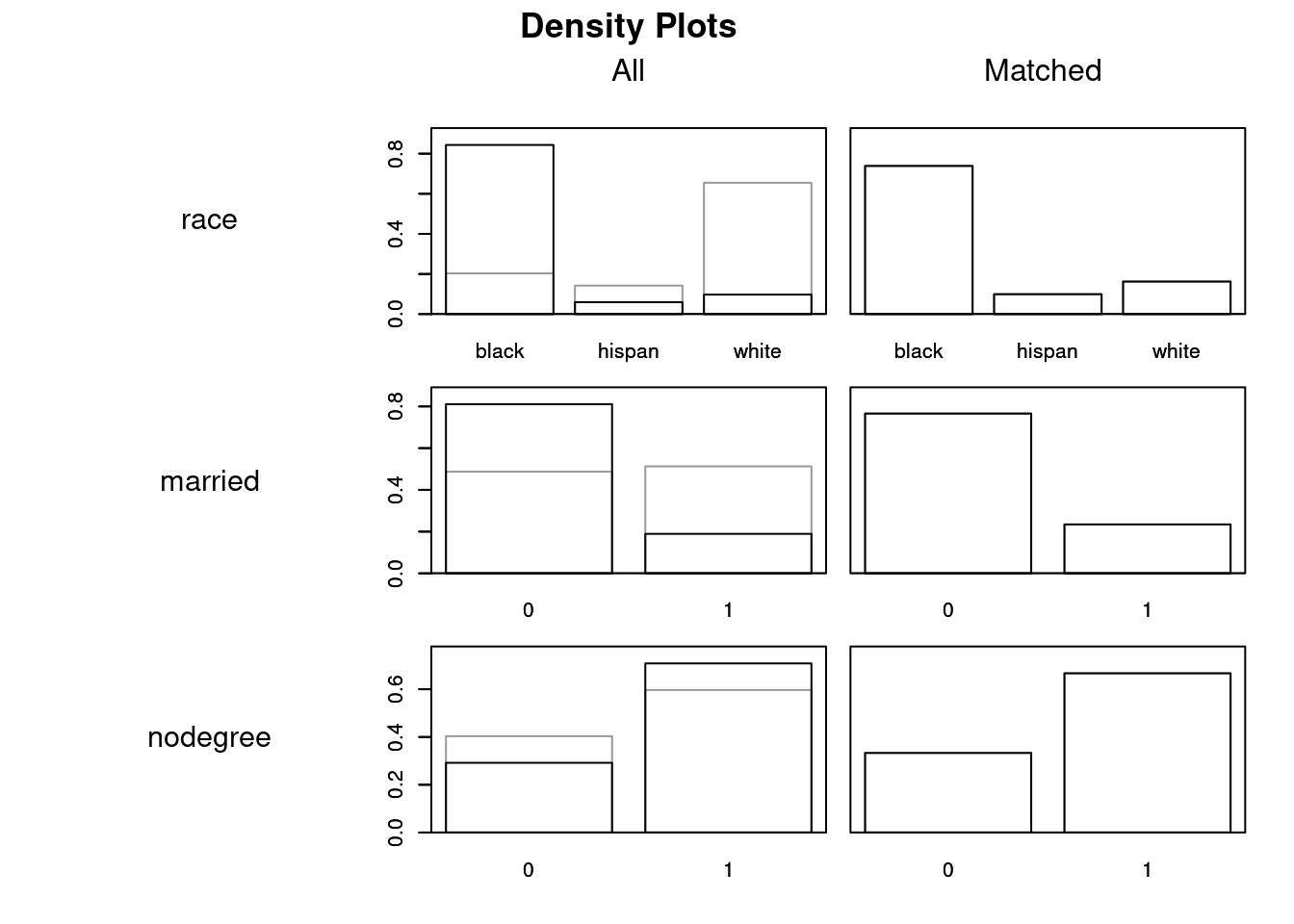
Question: What do you notice about the means of different covariates for the treated versus control groups?
In this case, we basically have perfect balance. This doesn’t always happen. Depending on the method and parameters you use, you could have “bad” matches where the covariates are unbalanced. If you conduct a matching and the covariate balance doesn’t look good, try another matching procedure!
2.2. Effect estimate
Here, we estimate linear regression models using the match data from 2.1 using the lm() function with the formula re78 ~ treat + race + married + nodegree and re78 ~ treat*(race + married + nodegree). The second linear model includes an interaction term. We pass weights that come from the matching. Notice that for this piece, we have passed the matched data match.data(exact_low). In the model without an interaction, the coefficient in front of the variable treat in the linear regression is our estimated effect. We can also simply compare the means of the two groups or calculate the parametric g-formulat by hand or by using from the ‘marginaleffects’ package. When using exact 1:1 matching and simple linear model, all estimates will agree.
If we use a different type of matching procedure, the estimates typically will not all be exactly the same. Additionally, if we use a more complicated model (such as the one with interactions) the causal effect will not correspond to a single coefficient from the linear model, but the parametric g-formula will still work.
fit <- lm(re78 ~ treat + race + married + nodegree,
          data = match.data(exact_low),
          w = weights)

coef(fit)
## (Intercept) treat racehispan racewhite married
## 6855.9543 379.9167 3264.0613 3070.2140 1795.8455
## nodegree
## -3022.6687
fit_int <- lm(re78 ~ treat*(race + married + nodegree),
          data = match.data(exact_low),
          w = weights)

coef(fit_int)
## (Intercept) treat racehispan
## 6517.07875 1057.66787 5175.55809
## racewhite married nodegree
## 4891.25175 1763.05130 -3229.92957
## treat:racehispan treat:racewhite treat:married
## -3822.99362 -3642.07549 65.58842
## treat:nodegree
## 414.52179
## parametric g-formula by hand from last week

## Get Actually treated individuals and set treatment to 0
d_all_control <- match.data(exact_low) %>%
  subset(treat == 1) %>% mutate(treat =0)

## Get Actually treated individuals
d_all_treat <- match.data(exact_low) %>%
  subset(treat == 1)

potential_outcomes_under_control <- predict(object = fit, newdata = d_all_control)
potential_outcomes_under_treatment <- predict(object = fit, newdata = d_all_treat)


# compare means of groups
mean(potential_outcomes_under_treatment) - mean(potential_outcomes_under_control)
## [1] 379.9167
# Take the average outcome for each group
match.data(exact_low) %>% group_by(treat) %>% summarise(mean = mean(re78))
## # A tibble: 2 × 2
## treat mean
## <int> <dbl>
## 1 0 6083.
## 2 1 6463.
## parametric g-formula using marginal effects
avg_comparisons(fit,
                variables = "treat",
                vcov = ~subclass,
                newdata = subset(treat == 1))
##
## Estimate Std. Error z Pr(>|z|) S 2.5 % 97.5 %
## 380 903 0.421 0.674 0.6 -1391 2151
##
## Term: treat
## Type: response
## Comparison: 1 - 0
potential_outcomes_under_control <- predict(object = fit_int, newdata = d_all_control)
potential_outcomes_under_treatment <- predict(object = fit_int, newdata = d_all_treat)

# compare means of groups
mean(potential_outcomes_under_treatment) - mean(potential_outcomes_under_control)
## [1] 379.9167
## parametric g-formula using marginal effects
avg_comparisons(fit_int,
                variables = "treat",
                vcov = ~subclass,
                newdata = subset(treat == 1))
##
## Estimate Std. Error z Pr(>|z|) S 2.5 % 97.5 %
## 380 898 0.423 0.672 0.6 -1379 2139
##
## Term: treat
## Type: response
## Comparison: 1 - 0Question: What is the estimated effect of job training on earnings?
3. Try it Yourself: Exact matching with high-dimensional confounding
3.1. Using matchit() to conduct a matching
Now suppose the adjustment set needs to also include 1974 earnings, re74. The adjustment set for this part is race, married, nodegree, and re74. Repeat exact matching as above.
# Your code goes hereQuestion: How many control units were matched? How many treated units?
3.2. Assessing the Match: Examining matched units
Look at the re74 values in the full data and among the matched units.
Here is one way to do this:
- Use the
select()function to get there74column in the full data. Pass this to thesummary()function to look at descriptive statistics of there74values in the full data. - Use the
select()function to get there74column in the matched data. Pass this to thesummary()function to look at descriptive statistics of there74values in the full data. You can get the matched data using thematch.datafunction.
Full data:
# your code goes hereMatched data:
# your code goes hereExplain what happened: What do you notice? What is different about the values of re74 in the full data versus the matched data? Explain what happened and why it happened. Briefly interpret the result from 3.2: what is the drawback of using exact matching in this setting?
3.3. Using matchit() to conduct a matching
Now suppose the adjustment set needs to also include 1974 earnings, re74. The adjustment set for this part is race, married, nodegree, and re74. Use nearest neighbor matching, but do not require exact matches. Instead pick a distance of your choice.
# use help to see what the various distances are
?matchit

# Your code goes here

non_exact_high <- matchit(treat ~ race + married + nodegree + re74,
                 data = lalonde,
                 method = "nearest",
                 estimand = "ATT",
                 distance = ...)